A Persistent Warm West in the Sundarbans of Bangladesh: Spatial Contrasts Are Recoverable Where Multi-Decadal Trends Are Not

Md. Imran Hossain; Md. Redwanur Rahman; Md. Mujibor Rahman; Md. Atiqur Rahman

doi:doi:10.11648/j.ajrs.20261402.18

Research Article |

| Peer-Reviewed

A Persistent Warm West in the Sundarbans of Bangladesh: Spatial Contrasts Are Recoverable Where Multi-Decadal Trends Are Not

Md. Imran Hossain

, Md. Redwanur Rahman^*

, Md. Mujibor Rahman

, Md. Atiqur Rahman

Published in American Journal of Remote Sensing (Volume 14, Issue 2)

Received: 17 September 2026 Accepted: 30 September 2026 Published: 20 October 2026

Views: Downloads:

Download PDF

Share This Article

Twitter
Linked In
Facebook

Abstract

The Bangladesh Sundarbans is the largest continuous mangrove forest in the world, and the satellite thermal record over it is now long enough to invite decadal analysis. We ask a prior question: which parts of that thermal signal can the archive actually resolve? Using 25 years of MODIS April composites, we find the western third of the forest persistently warmer than the eastern third, by 0.654°C on average (95% confidence interval +0.428 to +0.880°C, paired p = 3.6 × 10^-6) and in 23 of the 25 individual years. The west is also warmer than the centre in 24 of 25 years (+0.463°C), while centre and east are not reliably separable (+0.191°C, p = 0.052): the pattern is a warm west against a uniform remainder, not a gradient across the forest. The same record cannot support a trend. Sen’s slope for the whole forest is +0.039°C per year, with a confidence interval of −0.037 to +0.101 that contains zero, as does every sector interval; a Landsat 1995 to 2025 difference of +1.36°C rests on three sensor generations and on 13 against 29 contributing scenes. The asymmetry is structural rather than statistical: a contrast measured inside one composite shares its instrument, acquisition time, quality filter and mask on both sides, so those errors cancel, whereas a comparison between composites shares none of them. Two things follow. The western Sundarbans is repeatedly and measurably the warmest part of this forest, which is a target conservation can act on; and a record that cannot support a trend may still support a spatial result, so the two should not be reported with equal confidence.

Published in	American Journal of Remote Sensing (Volume 14, Issue 2)
DOI	10.11648/j.ajrs.20261402.18
Page(s)	134-151
Creative Commons	This is an Open Access article, distributed under the terms of the Creative Commons Attribution 4.0 International License (http://creativecommons.org/licenses/by/4.0/), which permits unrestricted use, distribution and reproduction in any medium or format, provided the original work is properly cited.
Copyright	Copyright © The Author(s), 2026. Published by Science Publishing Group

Keywords

Land Surface Temperature, MODIS, Mangrove Forest, Thermal Infrared Remote Sensing, Measurement Uncertainty, Google Earth Engine, Sen’s Slope

1. Introduction

Land surface temperature is among the most ecologically informative variables retrievable from thermal infrared sensors. It integrates solar irradiance, surface emissivity, land cover and evapotranspirative cooling into one measurable quantity

[1-3]

. Forest canopies are thermally distinctive within that signal, and the cooling effect of forest cover relative to surrounding surfaces is established at global scale

[4]

The satellite thermal record is now long enough to invite multi-decadal analysis, and warming trends derived from it are widely reported. A prior question receives far less attention. Given the instrument changes, sampling asymmetries and orbital drift embedded in a multi-decadal archive, which components of the thermal signal can that archive resolve?

The question has a structure, and the structure is geometric rather than statistical. Errors that accumulate along a long record — a sensor replacement, a change in the number of contributing scenes, a drifting overpass time, an inconsistent compositing window — propagate directly into any estimate of change over time. The same errors behave differently in a comparison made within a single image. If two parts of a forest are compared in the same composite, from the same instrument, under the same quality filter and the same water mask, then whatever the instrument was doing that year it was doing identically to both. The error does not propagate into the contrast. It cancels.

This distinction is rarely made explicit. Multi-decadal thermal studies commonly report a trend and a spatial pattern side by side as though the data supported both to the same degree. We use the Bangladesh Sundarbans to show that they do not, and that the difference is large enough to change which result a study should lead with.

The Bangladesh Sundarbans Reserved Forest is a useful case. It is the largest contiguous mangrove forest in the world. It is closed-canopy and structurally homogeneous over most of its extent, so a thermal contrast within it cannot be attributed to land-cover change. It sits under a documented west-to-east environmental gradient driven by freshwater delivery and salinity

[5, 6]

. It is cloud-prone, which constrains optical compositing in ways the analysis must confront rather than avoid. And it has been imaged continuously by MODIS since 2000 and by Landsat since the 1970s.

Thermal work on this forest exists. Rahman et al.

[7]

analysed 26 years of land surface temperature over the Bangladesh Sundarbans. They reported statistically significant cooling in February and December, land-cover change of approximately 5.78 km² yr⁻¹, and a clustering of dominant mangrove species by thermal regime, with Ceriops decandra associated with warmer zones and Heritiera fomes with cooler ones. A larger body of work treats Sundarbans land surface temperature as a response to land use and land cover change, predominantly on the Indian side of the border.

What has not been established for this forest is which components of the thermal signal the archive can resolve, and therefore which reported thermal results should be relied upon.

We address that directly. We partition the forest into three longitudinal sectors, measure the contrast between them within each annual MODIS composite, and test it across 25 paired years. We then apply the same archive to the trend question and report, with confidence intervals, what it can and cannot support.

The contribution is the demonstrated asymmetry between those two outcomes, together with the specific result that emerges from the first: a persistent western thermal anomaly of 0.654°C, sign-consistent in 23 of 25 years. We make no claim of priority. Whether some component of this pattern has been reported elsewhere does not affect the argument, which rests on a test that was run and a limitation that was characterised.

The specific objectives are:

to map the pre-monsoon thermal field of the forest at 30 m for four benchmark years;

to quantify the contrast between longitudinal sectors within each annual MODIS composite, and test it across 25 paired years;

to test for a monotonic trend in the same record and report its confidence interval;

to test for vegetation-temperature coupling at annual and pixel scale; and

to set out which of these results the measurement design supports.

2. Study Area and Data

2.1. The Bangladesh Sundarbans Reserved Forest

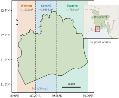
The Bangladesh Sundarbans Reserved Forest lies in the south-western coastal zone of Bangladesh between approximately 21°36′ and 22°30′ N and 89°02′ and 89°58′ E (Figure 1). It forms the Bangladeshi portion of the Sundarbans within the Ganges-Brahmaputra-Meghna delta. The analysis boundary used throughout this study encloses approximately 6,017 km².

The landscape is an intricate tidal creek network through which semi-diurnal tides from the Bay of Bengal regulate salinity, sediment flux and waterlogging. Dominant species include Heritiera fomes, Excoecaria agallocha and Sonneratia apetala, with composition varying systematically from west to east along a gradient in salinity and freshwater influence

[6]

The climate has three seasons: a cool dry winter from November to February, a hot pre-monsoon period from March to May, and a wet monsoon from June to October. The pre-monsoon carries the maximum surface thermal load, which is why it is the analytical window throughout this study.

Download: Download full-size image

Figure 1. The Bangladesh Sundarbans Reserved Forest and the three longitudinal sectors used in this study. Sector limits are the meridians 89.03°, 89.27°, 89.55° and 89.96° E; areas are approximate and are reported for scale only. The analysis boundary was digitised from a published cartographic source (Section 2.3). Country outlines in the locator inset are Natural Earth 1: 50 m, public domain. The sectors are geometric partitions and imply no salinity, ecological or administrative boundary.

2.2. Longitudinal Sectors, and What They Do Not Represent

The forest was partitioned into three sectors by intersecting the analysis boundary with three bounding rectangles in longitude: Western, 89.03°-89.27°E, approximately 1,192km²; Central, 89.27°-89.55° E, approximately 1,939 km²; and Eastern, 89.55°-89.96° E, approximately 1,768 km².

These are longitudinal sectors and nothing more. They are geometric partitions of the forest, not salinity zones, not ecological zones, and not administrative Forest Ranges. No salinity measurement was made or used anywhere in this study, and no salinity-based classification was applied.

We state this because the same longitudinal division appears in the regional literature under salinity labels. Adopting those labels would import an unmeasured variable into the study design, and would make any later reading of the thermal pattern as salinity-driven circular: geography would be labelled as salinity, and then the geographic pattern would be presented as evidence of salinity. The sector boundaries are identical to those used in a companion study of surface water dynamics in the same forest, which allows the two results to be compared directly.

2.3. Boundary Provenance and Positional Uncertainty

The analysis boundary was produced by georeferencing a published map of the Bangladesh Sundarbans Reserved Forest and digitising its outline. No authoritative vector boundary of the Reserved Forest was available to the authors at the time of analysis. The resulting polygon carries an unquantified positional error, likely largest along the northern margin where the forest abuts cultivation and aquaculture and where the forest-non-forest transition is gradational rather than sharp. Section 5.5 sets out which results this exposure affects and which it does not.

2.4. Satellite Data

Two products were used, chosen for their contrasting error structures rather than as a resolution-versus-coverage trade-off (Table 1).

Table 1. Satellite data used in this study.

Product	Resolution	Period	Band / variable	Quality control	Role
MODIS MOD11A2 V061	1 km, 8-day	2001-2025	LST_Day_1km	QC_Day bits 0-1 = 00; JRC water ≥ 50% masked	Sector contrast, trend, climatology
MODIS MOD13A3 V061	1 km, monthly	2001-2025	NDVI (× 0.0001)	JRC water ≥ 50% masked	NDVI pairing, climatology
Landsat 5 TM, C2 L2	30 m	1995, 2005	ST_B6	QA_PIXEL bits 3, 4; scene cloud ≤ 70%; NDWI ≥ 0 masked	Benchmark maps, differencing
Landsat 8 OLI/TIRS, C2 L2	30 m	2015, 2025	ST_B10	as above	Benchmark maps, differencing
Landsat 9 OLI-2/TIRS-2, C2 L2	30 m	2025	ST_B10	as above	Merged with Landsat 8 for 2025
JRC Global Surface Water	30 m	1984-2021	occurrence	—	Permanent water mask for MODIS

Landsat 7 ETM+ was excluded throughout because of the Scan Line Corrector failure. Conversions: MODIS LST (°C) = (DN × 0.02) − 273.15; Landsat LST (°C) = (DN × 0.00341802) + 149.0 − 273.15.

MODIS MOD11A2 Version 6.1

[8]

supplies eight-day composite land surface temperature at 1 km. One instrument covers the entire 2001-2025 record, so a comparison between parts of the forest within any given year carries no cross-sensor effect. This product carries the spatial analysis, which is the study’s primary result. MODIS MOD13A3 Version 6.1

[9]

supplies monthly NDVI on the same 1 km grid, allowing pixel-wise pairing without resampling.

Landsat Collection 2 Level-2 surface temperature supplies 30 m detail at four benchmark years, but spans three sensor generations across the record. It is used for spatial mapping and for map differencing, and its outputs are reported as observations rather than as trend estimates, for reasons developed in Section 5.1.

Permanent water was masked in the MODIS analyses using the JRC Global Surface Water occurrence layer

[10]

3. Methods

3.1. Analytical Design

All processing was performed in Google Earth Engine

[11]

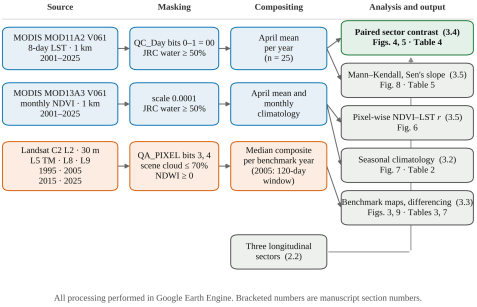
. Figure 2 sets out the full workflow: two source products, three masking paths, three compositing routes, and five analyses.

Download: Download full-size image

Figure 2. Processing and analysis workflow. Blue boxes are MODIS paths, orange boxes the Landsat path, and the green box the study’s primary analysis. Bracketed numbers refer to the section of this manuscript in which each step is described. All processing was performed in Google Earth Engine.

The design separates two questions that a single archive is usually asked to answer simultaneously. The first is spatial: does one part of the forest differ thermally from another? The second is temporal: is the forest as a whole changing? Section 5.1 explains why we treat these as distinct rather than as two views of the same measurement.

3.2. MODIS Processing

April composites of MOD11A2 V061 were retrieved for each year from 2001 to 2025. The LST_Day_1km band was converted to degrees Celsius as LST = (DN × 0.02) − 273.15. A pixel-level quality filter retained only observations with bits 0-1 of the QC_Day band equal to 00, which indicates good-quality retrieval without cloud contamination. Permanent water was masked using the JRC Global Surface Water occurrence layer at a threshold of ≥ 50% occurrence, which removes rivers, estuaries and major tidal channels. A pixel-level spectral water index was not used for MODIS because at 1 km it cannot resolve the tidal creek network.

All surviving eight-day composites within each April were averaged, and the result was reduced to a mean over each sector geometry and over the whole forest. Monthly NDVI was taken from MOD13A3 V061, scaled by 0.0001, and masked identically.

The number of eight-day composites contributing to each calendar month is not uniform across the record, and the departure matters for this study. MOD11A2 composites are assigned to a month by the calendar month of their start date, and the eight-day grid restarts on 1 January each year, so a month receives either three or four composite starts depending on where the grid falls. Over 25 years this yields 100 composites for most months, but 81 for April and October, 94 for May and November, and 99 for June (Table 2). April, the month on which every MODIS result in this study rests, has the fewest composites of any month — an average of 3.24 per year rather than 4. This is a property of the product’s compositing structure rather than a data fault, but it is reported rather than normalised because it bears on the precision of the annual means.

Table 2. Monthly climatology of land surface temperature and NDVI, Bangladesh Sundarbans, 2001-2025 (MODIS).

Month	Mean LST (°C)	Mean NDVI	Contributing 8-day composites (n)
Jan	21.20	0.691	100
Feb	24.51	0.677	100
Mar	28.03	0.655	100
Apr	29.72	0.622	81
May	29.71	0.594	94
Jun	29.12	0.574	99
Jul	28.92	0.584	100
Aug	27.92	0.633	100
Sep	28.37	0.722	100
Oct	27.52	0.740	81
Nov	25.47	0.736	94
Dec	21.98	0.707	100

1. LST range April − January = 8.52°C. NDVI range October − June = 0.166.

n is the number of MOD11A2 eight-day composites whose start date falls in that calendar month across the 25-year record. It is not uniform because the eight-day compositing grid restarts on 1 January each year, so a month receives three or four composite starts depending on where the grid falls. April, the analytical month for every annual result in this study, has the fewest.

Source: LST_NDVI_Combined_Climatology_Sundarbans_2001_2025.csv.

3.3. Landsat Processing

Pre-monsoon composites were built for 1995 and 2005 from Landsat 5 TM (band ST_B6), for 2015 from Landsat 8 OLI/TIRS (band ST_B10), and for 2025 from merged Landsat 8 and Landsat 9 scenes. Landsat 9 OLI-2/TIRS-2 was designed for radiometric and spectral continuity with Landsat 8

[12]

, which is the basis for merging the two within a single composite year. That continuity is a mission design objective verified at instrument level, not an independent validation for thermal retrievals over this surface.

Thermal values were converted using the USGS Collection 2 scaling, LST = (DN × 0.00341802) + 149.0 − 273.15. Cloud and cloud shadow were masked using bits 3 and 4 of the QA_PIXEL band, with a scene-level pre-filter excluding scenes above 70% cloud cover. Water was excluded by NDWI ≥ 0 computed from the atmospherically corrected green and near-infrared bands

[13]

, which follows the tidal creek network more faithfully than a static mask at 30 m. Surviving scenes were combined by median, which is more robust to residual haze than the mean at low scene counts

[14]

. Landsat 7 ETM+ was excluded throughout because of the Scan Line Corrector failure

[15]

The compositing windows are not identical across benchmark years, and the difference is material. 1995, 2015 and 2025 use 1 March - 30 April. 2005 uses 1 February - 31 May, a 120-day window rather than 61 days, extended because only one scene passed the cloud filter within the standard window. Climatological February in this forest is 24.51°C against 29.72°C in April (Table 2), so a window of that width samples a materially cooler part of the annual cycle. Section 5.5 quantifies the consequence.

3.4. The Paired Sector Design

The sector contrast was constructed as a paired comparison. For each year from 2001 to 2025, the Western, Central and Eastern sector means were extracted from the same annual composite, giving 25 matched triples. Differences were then formed within each year before any aggregation across years.

This ordering is the point of the design. Both members of each pair come from one instrument, one compositing window, one quality filter and one water mask, so any instrument state that varies between years is held constant within each pair and removed by the differencing. The design does not correct for those effects; it arranges the comparison so that they never enter it.

3.5. Statistical Analysis

Sector contrasts were tested with a paired t-test and with the Wilcoxon signed-rank test, the latter making no distributional assumption. Effect size is reported as Cohen’s dz and as a 95% confidence interval on the mean difference. Sign consistency is reported as the count of individual years in which the contrast holds, which is the most directly interpretable of the three and assumes nothing at all.

Monotonic trend was assessed by the Mann-Kendall test

[16, 17]

with Sen’s slope

[18]

. A 95% confidence interval on each slope was obtained from the rank-based variance of the Kendall S statistic. Reporting a confidence interval on a Sen’s slope, rather than a slope and a p-value alone, is central to this study’s argument and is done for every trend reported.

The test was applied to the raw annual series without prewhitening. Serial correlation can inflate the significance of Mann-Kendall results, and prewhitening is the usual remedy

[19]

. We did not apply it because no trend in this study is reported as significant, so the correction could only widen intervals that already contain zero and could not change any conclusion drawn here.

Vegetation-temperature coupling was tested at two scales: a Pearson correlation between the 25 annual April values of whole-forest LST and NDVI, and a pixel-wise Pearson correlation across the 25-image April stacks, computed in Earth Engine and exported as coefficient and p-value rasters.

All statistics were computed directly from the exported comma-separated tables and rasters, not from rounded values in any intermediate document.

4. Results

4.1. The Spatial Thermal Field

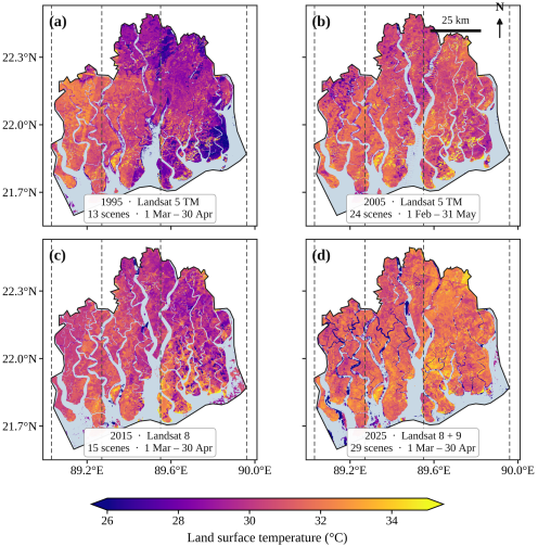
Landsat composites resolve the forest’s pre-monsoon thermal field at 30 m for all four benchmark years (Figure 3). Whole-forest mean LST was 29.91°C in 1995 from 13 scenes and 31.13°C in 2025 from 29 scenes, with 30.31°C in 2015 and 31.00°C in 2005 between them. Spatial standard deviations ranged from 2.26 to 2.96°C (Table 3).

Table 3. Landsat benchmark composite statistics, Bangladesh Sundarbans, pre-monsoon.

Year	Sensor	Acquisition window	Days	Scenes	Mean LST (°C)	SD (°C)
1995	Landsat 5 TM	1 Mar - 30 Apr	61	13	29.91	2.28
2005	Landsat 5 TM	1 Feb - 31 May	120	24	31.00	2.96
2015	Landsat 8 OLI/TIRS	1 Mar - 30 Apr	61	15	30.31	2.44
2025	Landsat 8 + Landsat 9	1 Mar - 30 Apr	61	29	31.13	2.26

The windows are not identical. The 2005 composite spans 120 days against 61 for the other three, extended because only one scene passed the cloud filter within the standard window. Climatological February is 24.51°C against 29.72°C in April (Table 2), so the 2005 composite is not thermally equivalent to the others.

Footnote on extreme values. Per-pixel extrema reach 74.92°C (1995), 69.90°C (2005), 65.75°C (2015) and 63.31°C (2025); minima reach −44.32, −60.61, −49.08 and −26.14°C respectively. These are residual cloud-edge and unmasked-water pixels, not surface temperatures. They are disclosed rather than removed because no documented clipping procedure exists for this dataset; the reported means are computed over the full valid-pixel population including them.

Source: GEE console output, Screenshots 1315, 1316, 1344, 1345.

Two features are visible in every panel. The tidal creek network appears as masked gaps, confirming that the NDWI water mask follows the channel system rather than a static outline. And the western third of the forest reads consistently warmer than the eastern third, in composites built from three different sensors. That visual pattern is what Section 4.2 tests.

Download: Download full-size image

Figure 3. Landsat Collection 2 Level-2 pre-monsoon land surface temperature for the four benchmark years, at 30 m, on a common colour scale. Pale blue marks water and cloud pixels removed by the NDWI and QA_PIXEL masks. Dashed lines mark the sector boundaries of Figure 1. Each panel states its sensor, scene count and compositing window; note that panel (b) uses a 120-day window while the other three use 61 days (Section 3.3).

4.2. A Persistent Western Thermal Anomaly

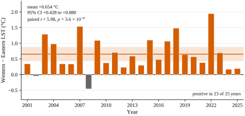
The Western sector is warmer than the Eastern sector by a mean of 0.654°C, with a 95% confidence interval of +0.428 to +0.880°C, and the difference is positive in 23 of the 25 individual years. Tested as a paired comparison across years, t = 5.98 with 24 degrees of freedom, p = 3.6 × 10^-6; the Wilcoxon signed-rank test gives W = 12.0, p = 4.2 × 10^-6. The standardised effect size is dz = 1.20.

Across the record, the 25-year grand mean April LST was 29.82°C in the Western sector, 29.35°C in the Central sector and 29.16°C in the Eastern sector (Table 4). Paired contrasts for all three sector pairs are given in Table 5, and the full annual series in Table 6.

Table 4. Sector summary statistics, April 2001-2025 (MODIS MOD11A2).

Sector	Grand mean (°C)	SD (°C)	Sen’s slope (°C yr⁻¹), 95% CI	τ	p
Western	29.82	0.92	+0.034 (−0.008, +0.102)	0.240	0.098
Central	29.35	0.99	+0.043 (−0.015, +0.106)	0.200	0.170
Eastern	29.16	1.11	+0.029 (−0.055, +0.109)	0.100	0.502
Whole forest	29.37	1.00	+0.039 (−0.037, +0.101)	0.173	0.236

2. Sector longitude limits are given in Table 1 and Figure 1. τ is Kendall’s tau.

Every slope confidence interval contains zero.

Table 5. Paired sector contrasts across 25 years, April 2001-2025 (MODIS MOD11A2).

Contrast	Mean difference (°C), 95% CI	Years positive	Paired t	p	Wilcoxon p	dz
Western − Eastern	+0.654 (+0.428, +0.880)	23 / 25	5.98	3.6 × 10^-6	4.2 × 10^-6	1.20
Western − Central	+0.463 (+0.339, +0.587)	24 / 25	7.72	5.9 × 10^-8	1.2 × 10^-7	1.54
Central − Eastern	+0.191 (−0.002, +0.384)	15 / 25	2.04	0.052	0.063	0.41

Table 6. Annual April mean LST by sector and for the whole forest, 2001-2025 (°C).

Year	Western	Central	Eastern	Whole forest	W − E
2001	30.78	30.38	30.44	30.48	+0.34
2002	27.89	27.34	27.93	27.69	−0.04
2003	29.44	28.96	28.15	28.77	+1.29
2004	27.95	28.09	26.97	27.62	+0.98
2005	29.58	29.24	29.23	29.31	+0.34
2006	29.80	29.27	29.47	29.46	+0.34
2007	29.34	28.23	27.80	28.23	+1.54
2008	29.54	29.11	30.00	29.56	−0.45
2009	30.06	29.66	28.97	29.47	+1.09
2010	29.77	29.24	29.40	29.40	+0.37
2011	29.69	29.34	28.99	29.30	+0.71
2012	30.35	29.95	30.12	30.10	+0.23
2013	30.21	29.82	29.62	29.82	+0.59
2014	31.38	31.07	31.08	31.14	+0.30
2015	29.47	28.21	28.37	28.56	+1.10
2016	30.47	30.14	29.99	30.15	+0.48
2017	29.42	28.93	28.36	28.79	+1.07
2018	29.68	28.82	28.20	28.76	+1.48
2019	30.03	29.55	29.39	29.58	+0.64
2020	29.90	29.46	29.33	29.51	+0.57
2021	29.68	29.53	29.30	29.47	+0.38
2022	29.80	28.90	27.85	28.65	+1.95
2023	31.14	30.92	30.45	30.78	+0.69
2024	31.74	31.55	31.57	31.59	+0.17
2025	28.29	28.10	28.10	28.12	+0.19
Mean	29.82	29.35	29.16	29.37	+0.654
SD	0.92	0.99	1.11	1.00	0.547

Whole-forest values are computed over the full boundary polygon and are not the arithmetic mean of the three sectors, which differ in area.

Source: LST_Zonal_Annual_…csv and NDVI_LST_Annual_…csv.

Standard deviations of the differences are 0.547, 0.300 and 0.468°C respectively. Wilcoxon signed-rank statistics are W = 12.0, 1.0 and 93.0.

Strict three-way ordering Western > Central > Eastern holds in 14 of 25 years (56%).

Each pair is measured within the same annual composite, from the same instrument, under the same quality filter and the same water mask. Degrees of freedom = 24 throughout.

Source: LST_Zonal_Annual_Sundarbans_2001_2025.csv. Cross-check: the grand means reproduce the independently exported ee-chart (9).csv (29.816418 / 29.353513 / 29.162372) exactly.

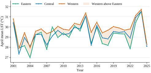
Interannual variation is far larger than the separation between sectors: the whole-forest annual mean ranges over 3.98°C, with a standard deviation of 0.995°C. The Western series nevertheless sits above the other two in almost every year (Figure 4).

Download: Download full-size image

Figure 4. April mean land surface temperature by sector, 2001-2025, from MODIS MOD11A2 at 1 km after quality filtering and permanent-water masking. Shading marks years in which the Western sector exceeds the Eastern sector, which is 23 of the 25 years. All three sectors track the same large interannual variability while the Western series remains above the other two.

The Western-Central contrast is smaller in magnitude but more consistent still: mean +0.463°C (95% CI +0.339 to +0.587), positive in 24 of 25 years, t = 7.72, p = 5.9 × 10^-8, Wilcoxon p = 1.2 × 10^-7, dz = 1.54.

The two years in which the Western sector was not the warmest were 2002, at −0.043°C, and 2008, at −0.454°C (Figure 5). Both margins are small against the record’s interannual spread.

Download: Download full-size image

Figure 5. Western minus Eastern sector April mean LST for each year, 2001-2025. Each bar is a difference measured within a single annual composite, from one instrument, under one quality filter and one water mask. The horizontal line and shaded band are the mean difference and its 95% confidence interval. Grey bars mark the two years in which the difference is negative.

4.3. An Anomaly, Not a Gradient

The Central sector exceeds the Eastern sector by a mean of 0.191°C, with a 95% confidence interval of −0.002 to +0.384°C, positive in 15 of 25 years, t = 2.04, p = 0.052, Wilcoxon p = 0.063, dz = 0.41. The interval includes zero and the sign consistency is barely better than chance.

The strict three-way ordering Western > Central > Eastern holds in only 14 of 25 years, or 56%.

These results describe a western anomaly set against a comparatively uniform central-eastern forest, not a monotonic west-to-east gradient. That is a narrower claim than a three-step gradient and a more falsifiable one, and it is what the data support.

4.4. No Vegetation-Temperature Coupling Detected

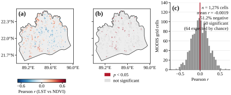
Annual April NDVI and LST across 2001-2025 are essentially uncorrelated: Pearson r = +0.055, p = 0.794, n = 25 (Table 7).

Table 7. Annual April mean NDVI and LST, whole forest, 2001-2025 (MODIS).

Year	NDVI	LST (°C)	Year	NDVI	LST (°C)
2001	0.620	30.48	2014	0.619	31.14
2002	0.646	27.69	2015	0.611	28.56
2003	0.638	28.77	2016	0.608	30.15
2004	0.571	27.62	2017	0.628	28.79
2005	0.609	29.31	2018	0.653	28.76
2006	0.628	29.46	2019	0.640	29.58
2007	0.622	28.23	2020	0.664	29.51
2008	0.586	29.56	2021	0.633	29.47
2009	0.586	29.47	2022	0.618	28.65
2010	0.576	29.40	2023	0.671	30.78
2011	0.635	29.30	2024	0.634	31.59
2012	0.610	30.10	2025	0.661	28.12
2013	0.594	29.82

3. Pearson r = +0.055, p = 0.794, n = 25. No significant temporal association.

Pixel-wise across 1,276 valid 1 km grid cells: mean r = −0.0019, 51.2% negative; 50 cells reach p < 0.05 where 63.8 would be expected by chance alone; of those 50, 28 are negative and 22 positive, with a mean coefficient of −0.048. Source: NDVI_LST_Correlation_Map_2001_2025.tif and NDVI_LST_Pvalue_Map_2001_2025.tif.

The pixel-wise analysis gives the same answer more sharply (Figure 6). Across 1,276 valid MODIS grid cells, the mean Pearson r between the 25-image April LST and NDVI stacks is −0.0019, with 51.2% of cells negative and 48.8% positive — indistinguishable from a random split. Fifty cells reach p < 0.05, which is 3.9% of the total; 63.8 would be expected at that threshold by chance alone in the absence of any relationship. Of the 50, twenty-eight are negative and twenty-two positive, and their mean coefficient is −0.048.

Fewer cells reach significance than chance alone would produce. This is a null result and is reported as one. NDVI in this closed-canopy forest spans roughly 0.57 to 0.74 across the seasonal cycle, and considerably less across space within any one month. There may simply be insufficient variance in canopy density to drive a detectable thermal response at 1 km. Strong negative NDVI-LST relationships are typically recovered in landscapes containing large contrasts between vegetated and impervious or bare surfaces

[20, 21]

, a condition a closed-canopy mangrove forest does not meet. That explanation is plausible but was not tested here, and we do not claim it. The finding is that no coupling was detected under this design.

Download: Download full-size image

Figure 6. Pixel-wise relationship between April LST and April NDVI, 2001-2025, at 1 km. (a) Pearson correlation coefficient. (b) Cells reaching p < 0.05, in red. (c) Distribution of the coefficient across all 1,276 valid cells; the vertical red line is the mean. Fifty cells reach significance where 64 would be expected by chance alone, so the analysis detects no coupling at this scale.

4.5. Seasonal Amplitude Sets the Scale

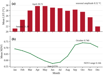
Monthly climatology across 2001-2025 places the LST maximum in April at 29.72°C and the minimum in January at 21.20°C, a seasonal amplitude of 8.52°C (Figure 7; Table 2). NDVI runs inversely, from a June minimum of 0.574 to an October maximum of 0.740, a range of 0.166, lagging the thermal cycle by approximately two months.

This pattern is the monsoon signal, shared by every vegetated surface in the delta, and we make no ecological claim from it. Its function here is quantitative. It establishes that the shared seasonal forcing has an amplitude of 8.52°C, against which the 0.654°C spatial residual between sectors is small. A contrast of that size is detectable only because it is measured between sectors experiencing the same forcing in the same image.

Download: Download full-size image

Figure 7. Monthly climatology of (a) land surface temperature and (b) NDVI, 2001-2025, from MODIS MOD11A2 and MOD13A3. The two variables are shown on separate panels sharing a month axis rather than on a shared dual axis, because on a dual axis the apparent crossing point of the two curves is set by the choice of scales and carries no information.

4.6. The Multi-Decadal Trend Is Not Resolvable

Whole-forest April mean LST averaged 29.37°C across 2001-2025 and ranged from 27.62°C in 2004 to 31.60°C in 2024, an interannual range of 3.98°C and a standard deviation of 0.995°C (Table 6). The three coldest years in the record were 2004 at 27.62°C, 2002 at 27.69°C and 2025 at 28.12°C.

Whole-forest values are computed over the full boundary polygon and are not the arithmetic mean of the three sectors, which differ in area.

Source: LST_Zonal_Annual_…csv and NDVI_LST_Annual_…csv.

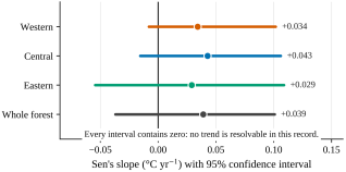
Sen’s slope for the whole forest is +0.039°C yr⁻¹ with a 95% confidence interval of −0.037 to +0.101; Kendall’s τ = 0.173, p = 0.236. Per sector: Western +0.034 (95% CI −0.008 to +0.102, τ = 0.240, p = 0.098), Central +0.043 (95% CI −0.016 to +0.106, τ = 0.200, p = 0.170) and Eastern +0.029 (95% CI −0.055 to +0.109, τ = 0.100, p = 0.502).

Every one of these confidence intervals contains zero (Figure 8). The interannual standard deviation of the whole-forest mean, 0.995°C, exceeds the entire 25-year change implied by the central slope estimate. No trend is resolvable in this record, and we do not report one. The ordering of four non-significant slopes is not interpreted.

Download: Download full-size image

Figure 8. Sen’s slope estimates for April mean LST, 2001-2025, with 95% confidence intervals derived from the rank-based variance of the Kendall S statistic. Every interval contains zero, at every spatial aggregation.

4.7. Landsat Map Differences, Reported as Observations

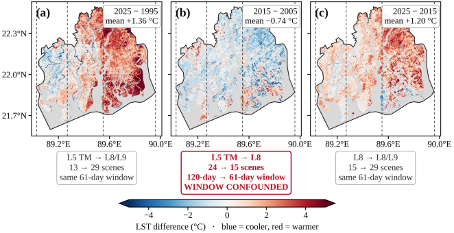
Pixel-wise differencing over the intersection of valid pixels gives a mean of +1.36°C for 2025 − 1995, −0.74°C for 2015 − 2005 and +1.20°C for 2025 − 2015 (Figure 9; Table 8). Warmed area was 3,483.64 km² against 991.85 km² cooled over the 30-year pair, 1,344.57 km² against 2,880.27 km² for the middle decade, and 3,434.78 km² against 808.60 km² for the recent decade.

Table 8. Landsat LST map differences between benchmark composites (30 m).

Period	Mean (°C)	P10 (°C)	P90 (°C)	Warmed (km²)	Cooled (km²)	Footprint (km²)	% warmed
2025 − 1995	+1.36	−1.23	+4.23	3,483.64	991.85	4,475.49	77.8
2015 − 2005 †	−0.74	−2.40	+1.42	1,344.57	2,880.27	4,224.84	31.8
2025 − 2015	+1.20	−0.72	+3.23	3,434.78	808.60	4,243.38	80.9

These are map differences between composites, not trend estimates, and their magnitudes are not interpreted as measures of climatic warming. Each spans one or more sensor transitions and unequal scene counts. No uncertainty estimate accompanies them.

† The 2005 baseline uses a 120-day compositing window (Table 3). The net cooling in this period may be partly or wholly an artefact of that window difference, and this study cannot separate the two. This row should not be used.

Footprints differ between periods because the intersection of valid pixels differs; percentages are computed against each period’s own footprint. P10 and P90 are the 10th and 90th percentiles of the per-pixel change distribution.

Source: GEE console output, Screenshots 1344-1348, read first-hand.

These are map differences, not trends, and we do not interpret their magnitude as a measure of climatic warming. Each spans one or more sensor transitions. The 1995 composite rests on 13 scenes against 29 for 2025. The 2005 composite uses a 120-day window against 61 days for the others. The overpass time is not constant across the record. No uncertainty estimate accompanies them, and none can be produced from the outputs available.

The valid-pixel footprints differ between periods, at 4,475.49, 4,224.84 and 4,243.38 km² respectively, because the intersection of valid pixels differs. Percentages are therefore reported against each period’s own footprint: 77.8%, 31.8% and 80.9% warmed.

Download: Download full-size image

Figure 9. Landsat LST map differences for three benchmark periods, at 30 m. The confounds attaching to each pair are printed beneath the panel. Panel (b) is flagged because its 2005 baseline uses a 120-day compositing window against 61 days for its comparator, and this is also the only period showing net cooling; that result should not be used (Section 5.5). Grey marks pixels invalid in either composite of the pair.

5. Discussion

5.1. Why One Comparison Survives and the Other Does Not

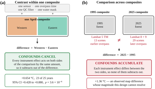
The two headline quantities in this study — a 0.654°C spatial contrast and a +1.36°C map difference — are similar in magnitude. They are not similar in how well the data support them, and the reason is structural rather than statistical (Figure 10).

Consider what would have to be true for the spatial contrast to be an artefact. The instrument, in a single composite on a single set of days, would have to have measured the Western sector systematically warmer than the Eastern one for a reason unrelated to the surface. The same sensor made both measurements. The same quality filter passed both. The same water mask was applied to both. Whatever the overpass time was that year, it was that time for both. Whatever calibration state the instrument was in, it was in that state for both. No mechanism in the sensor chain acts on one longitude band of a single image and not the adjacent one. Were such a mechanism to exist, it would have to act in the same direction in 23 of 25 independent years to produce this result.

Now consider the map difference. It compares a Landsat 5 TM composite from 1995 with a Landsat 8/9 composite from 2025. These are different instruments with different band passes and different calibration histories, and TIRS in particular carried a documented stray-light problem addressed only through subsequent processing development

[22, 23]

. Collection 2 applies a consistent processing chain to both, but consistent processing is not equivalent measurement. The 1995 composite rests on 13 scenes and the 2025 composite on 29, so the two medians are not equally well determined. Landsat’s descending-node crossing has drifted later across this record, and surface temperature is more sensitive to acquisition time than almost any other retrievable variable. None of these effects cancel. All of them accumulate into the difference. A +1.36°C result across that stack of confounds is not obviously a signal, and we cannot demonstrate that it is one.

The MODIS trend is subject to a milder version of the same problem, and fails for a simpler reason: its confidence interval contains zero, and the interannual standard deviation exceeds the implied 25-year change.

Download: Download full-size image

Figure 10. Why the two comparisons behave differently. (a) A contrast measured between sectors within one composite: every instrument effect acts on both sides by the same amount and subtracts out of the difference. (b) A comparison between composites: the instrument, the scene count and the overpass time all differ between the two sides, so none of those effects subtracts out. The geometry of the comparison, not the length of the record, determines which result the archive can support.

The general point is that a long archive is not uniformly informative. It supports comparisons whose confounds cancel and fails to support comparisons whose confounds accumulate. Which of those a given result is depends on the geometry of the comparison rather than on the length of the record. Reporting both at equal confidence, as is common in this literature, misstates what the data show.

5.2. What Might Produce a Persistent Western Anomaly

We have demonstrated the anomaly and not its cause, and the distinction is worth keeping sharp. What follows is candidate explanation, not result.

The most plausible candidate is the west-to-east environmental gradient that structures this forest. Reduced dry-season freshwater delivery through the western distributary system, associated with upstream abstraction, has been linked to elevated salinity in the western Sundarbans

[5]

. Increased salinity has in turn been associated with changes in plant community composition and condition across this forest

[6]

. A canopy under chronic salt stress, with reduced leaf area and lower stomatal conductance, would convert a greater fraction of absorbed radiation to sensible rather than latent heat, raising surface temperature. That mechanism is consistent with our observation and would predict the pattern we see.

No salinity was measured in this study, and no canopy physiological variable was measured. The mechanism is therefore offered as a hypothesis the data are consistent with, not as a finding. Our own NDVI analysis (Section 4.4) provides no support for the vegetation-density limb of that chain: no LST-NDVI coupling was detected at annual or pixel scale. That absence is as likely to reflect NDVI’s insensitivity in closed canopy as the absence of the mechanism, but it means we cannot use our own data to close the argument.

Independent support arrives from a different direction. Rahman et al.

[7]

, analysing the same forest, found dominant mangrove species clustering by thermal regime, with the salt-tolerant Ceriops decandra associated with warmer zones and the freshwater-preferring Heritiera fomes with cooler ones. Because those species are distributed along the west-to-east salinity gradient, their result implies a spatial thermal pattern consistent with ours, reached through a different partition of the forest and a different method. Two independent approaches converging on the same spatial structure is meaningful. Neither establishes the mechanism.

5.3. Convergence with an Independent Variable

A companion study of the same forest examined dry-season surface water dynamics across the Landsat record, using the identical sector boundaries. It reached a structurally identical conclusion: the multi-decadal trend was not resolvable, while spatially and event-referenced contrasts were. Two different variables, two different products, the same archive, the same forest, and the same finding about what is recoverable.

This bears on generality. A single-site methodological claim invites the response that the site is peculiar. A claim that holds for two independent variables measured over the same site is harder to dismiss as an artefact of one measurement chain. It remains a single-site result, and we do not extend it further.

5.4. Implications for Thermal Monitoring

If the recoverable signal in this archive is spatial, monitoring designs should be built around spatial contrasts rather than trend estimation. A programme tracking thermal stress in the Sundarbans would learn more from repeated within-scene sector comparisons than from extending a trend line. Those comparisons are cheap, robust and interpretable year on year; the trend line’s confidence interval will continue to contain zero for the foreseeable record.

The management-relevant result is also spatial rather than temporal. The Western sector is persistently the warmest part of this forest, in almost every year, and it is the same sector identified in the regional literature as facing the greatest salinity pressure. That is an actionable targeting statement. “The forest warmed by 1.4°C” is not, both because we cannot substantiate it and because it implies no spatial priority.

5.5. Limitations

No uncertainty assessment accompanies the Landsat composites. No cross-sensor bias assessment, overlap-period comparison or accuracy validation was performed, and none can be produced from the existing outputs. This is why Section 4.7 reports observations rather than estimates.

The compositing windows are unequal, and one result is unusable because of it. The 2005 composite spans 1 February - 31 May, twice the length of the other three. Climatological February is 24.51°C against 29.72°C in April, so that window samples a materially cooler part of the annual cycle. 2005 is the baseline of the 2015 − 2005 pair, which is the one period showing net cooling. That cooling may be partly or wholly an artefact of the window difference, and this study cannot separate the two. The 2015 − 2005 result should not be used.

Observation depth is unequal and per-pixel counts were not retained. The Landsat composites rest on 13, 24, 15 and 29 scenes. A median over 13 scenes across four path/rows is thin.

Overpass drift was not characterised, for either the Landsat descending-node crossing or Terra’s orbital drift. Both affect the trend estimate. Neither affects a within-scene contrast, for the reasons in Section 5.1. Spatial sampling uncertainty in MODIS Terra LST retrievals is itself non-trivial and was not propagated here

[24]

; it too acts on both sides of a within-scene contrast.

The detection floor was not characterised. No power analysis was performed for the null NDVI-LST result, so we cannot state how large a correlation this design could have detected. Section 4.4 therefore reports “not detected under this design” rather than “absent”. The same caution applies to the Central-Eastern contrast, which is not significant but is also not demonstrated to be zero.

April has the fewest composites of any month, 81 over 25 years rather than 100 (Section 3.2). The annual April means are correspondingly slightly less well determined than a reader might assume.

Artefact pixels remain in the Landsat composites. Per-pixel extrema reach 74.92°C and −60.61°C (Table 3, footnote). These are residual cloud-edge and unmasked-water pixels, not surface temperatures. They are retained in the reported means because a post-hoc clip could not be documented, and an undocumented clip is worse than a disclosed artefact. Their effect on a mean over several million pixels is small but is not formally bounded.

The analysis boundary carries unquantified positional error (Section 2.3), greatest at the northern margin. The northern margin is also where the 30-year change map shows its strongest warming, so that particular feature is the one least separable from boundary error, and we place no weight on it. The sector contrast is far less exposed. It is computed over sector interiors containing thousands of 1 km cells. A boundary error would have to be both large and systematically asymmetric between sectors to generate a 0.654°C difference sustained across 23 of 25 years.

All results come from one forest. The methodological argument is expected to generalise to other multi-decadal optical thermal records over spatially structured, cloud-prone canopies, but that expectation is untested here. Comparable multi-sensor records of similar length exist for other parts of Bangladesh, including a 25-year analysis of rainfall-surface temperature coupling and compound dry-hot persistence over the northwest of the country

[25]

, and such records offer a direct setting in which to test it.

6. Conclusions

In a multi-decadal optical satellite record over a tidal mangrove forest, the recoverable thermal signal is spatial rather than temporal. Twenty-five years of MODIS observations over the Bangladesh Sundarbans resolve a persistent thermal anomaly in the western part of the forest. The Western sector is warmer than the Eastern by 0.654°C on average, with a 95% confidence interval of +0.428 to +0.880°C, and warmer in 23 of 25 individual years. It is warmer than the Central sector in 24 of 25. Central and Eastern are not reliably separable. The forest’s thermal structure is a western anomaly against a comparatively uniform remainder, not a west-to-east gradient.

The same archive does not resolve a multi-decadal trend. Sen’s slope for the whole forest is +0.039°C yr⁻¹ with a confidence interval spanning zero, every sector interval also contains zero, and the interannual standard deviation of the annual mean exceeds the implied 25-year change. The Landsat 1995→2025 map difference of +1.36°C spans three sensor generations, unequal scene counts, unequal compositing windows and an unassessed overpass drift; we report it as an observed map difference and decline to interpret its magnitude.

No vegetation-temperature coupling was detected at annual or pixel scale. Fewer grid cells reached significance than chance alone would produce.

The asymmetry between these outcomes is the study’s main point. A contrast measured between parts of the same image inherits none of the confounds that accumulate along a multi-decadal record, because the instrument state, the acquisition time, the quality filter and the mask are shared by both sides of the comparison. Where an archive supports a spatial result and not a temporal one, saying so is more useful than reporting both at equal confidence. In this case the spatial result is also the one with management value: the western Sundarbans is reliably the warmest part of this forest, and that is a statement a conservation programme can act on.

Abbreviations

CI	Confidence Interval
DN	Digital Number
ETM+	Enhanced Thematic Mapper Plus
GEE	Google Earth Engine
JRC	Joint Research Centre
LST	Land Surface Temperature
MODIS	Moderate Resolution Imaging Spectroradiometer
NDVI	Normalized Difference Vegetation Index
NDWI	Normalized Difference Water Index
OLI	Operational Land Imager
QA	Quality Assurance
SD	Standard Deviation
SLC	Scan Line Corrector
TIRS	Thermal Infrared Sensor
TM	Thematic Mapper

Author Contributions

Md. Imran Hossain: Conceptualization, Data curation, Formal Analysis, Methodology, Software, Visualization, Writing – original draft

Md. Redwanur Rahman: Supervision, Validation, Writing – review & editing

Md. Mujibor Rahman: Validation, Writing – review & editing

Md. Atiqur Rahman: Investigation, Resources

Data Availability Statement

All satellite products used in this study are publicly available. MOD11A2 Version 6.1 and MOD13A3 Version 6.1 are distributed by the NASA Land Processes Distributed Active Archive Center

[8, 9]

; Landsat Collection 2 Level-2 surface temperature is distributed by the United States Geological Survey; and the Global Surface Water dataset is distributed by the European Commission Joint Research Centre

[10]

. Country outlines in Figure 1 are Natural Earth 1: 50 m, public domain.

The Google Earth Engine scripts implementing all analyses, the Python code that generates every figure from the exported tables and rasters, and the derived tabular outputs supporting all results are available from the authors upon reasonable request.

Conflicts of Interest

The authors declare no conflicts of interest.

References

[1]	Wan, Z. New refinements and validation of the MODIS Land-Surface Temperature/Emissivity products. Remote Sensing of Environment. 2008, 112(1), 59-74. https://doi.org/10.1016/j.rse.2006.06.026
[2]	Weng, Q. Thermal infrared remote sensing for urban climate and environmental studies: Methods, applications, and trends. ISPRS Journal of Photogrammetry and Remote Sensing. 2009, 64(4), 335-344. https://doi.org/10.1016/j.isprsjprs.2009.03.007
[3]	Li, Z.-L., Tang, B.-H., Wu, H., Ren, H. Satellite-derived land surface temperature: Current status and perspectives. Remote Sensing of Environment. 2013, 131, 14-37. https://doi.org/10.1016/j.rse.2012.12.008
[4]	Mildrexler, D. J., Zhao, M., Running, S. W. A global comparison between station air temperatures and MODIS land surface temperatures reveals the cooling role of forests. Journal of Geophysical Research: Biogeosciences. 2011, 116, G03025. https://doi.org/10.1029/2010JG001486
[5]	Rahman, M. M., Rahaman, M. M. Impacts of Farakka barrage on hydrological flow of Ganges river and environment in Bangladesh. Sustainable Water Resources Management. 2017, 4(4), 767-780. https://doi.org/10.1007/s40899-017-0163-y
[6]	Rahman, M. M. Impact of increased salinity on the plant community of the Sundarbans Mangrove of Bangladesh. Community Ecology. 2020, 21(3), 273-284. https://doi.org/10.1007/s42974-020-00028-1
[7]	Rahman, R-R., Rakib, M. I. H., Ahmed, A., Tabassum, T., Sorker, R., Alam, M. Assessing the vulnerability of Sundarbans mangroves to LST variability: Utilising 26-year spatiotemporal data. International Journal of Climatology. 2026, 46(7), e70372. https://doi.org/10.1002/joc.70372
[8]	Wan, Z., Hook, S., Hulley, G. MOD11A2 MODIS/Terra Land Surface Temperature/Emissivity 8-Day L3 Global 1 km SIN Grid V061 [Dataset]. NASA EOSDIS Land Processes DAAC, 2021. https://doi.org/10.5067/MODIS/MOD11A2.061
[9]	Didan, K. MOD13A3 MODIS/Terra Vegetation Indices Monthly L3 Global 1 km SIN Grid V061 [Dataset]. NASA EOSDIS Land Processes DAAC, 2021. https://doi.org/10.5067/MODIS/MOD13A3.061
[10]	Pekel, J.-F., Cottam, A., Gorelick, N., Belward, A. S. High-resolution mapping of global surface water and its long-term changes. Nature. 2016, 540(7633), 418-422. https://doi.org/10.1038/nature20584
[11]	Gorelick, N., Hancher, M., Dixon, M., Ilyushchenko, S., Thau, D., Moore, R. Google Earth Engine: Planetary-scale geospatial analysis for everyone. Remote Sensing of Environment. 2017, 202, 18-27. https://doi.org/10.1016/j.rse.2017.06.031
[12]	Masek, J. G., Wulder, M. A., Markham, B., McCorkel, J., Crawford, C. J., Storey, J., Jenstrom, D. T. Landsat 9: Empowering open science and applications through continuity. Remote Sensing of Environment. 2020, 248, 111968. https://doi.org/10.1016/j.rse.2020.111968
[13]	McFeeters, S. K. The use of the Normalized Difference Water Index (NDWI) in the delineation of open water features. International Journal of Remote Sensing. 1996, 17(7), 1425-1432. https://doi.org/10.1080/01431169608948714
[14]	Flood, N. Seasonal composite Landsat TM/ETM+ images using the medoid (a multi-dimensional median). Remote Sensing. 2013, 5(12), 6481-6500. https://doi.org/10.3390/rs5126481
[15]	Wulder, M. A., Loveland, T. R., Roy, D. P., Crawford, C. J., Masek, J. G., Woodcock, C. E., Allen, R. G., Anderson, M. C., Belward, A. S., Cohen, W. B., Dwyer, J., Erb, A., Gao, F., Griffiths, P., Helder, D., Hermosilla, T., Hipple, J. D., Hostert, P., Hughes, M. J., Zhu, Z. Current status of Landsat program, science, and applications. Remote Sensing of Environment. 2019, 225, 127-147. https://doi.org/10.1016/j.rse.2019.02.015
[16]	Mann, H. B. Nonparametric tests against trend. Econometrica. 1945, 13(3), 245-259. https://doi.org/10.2307/1907187
[17]	Kendall, M. G. Rank Correlation Methods, 4th ed. London: Charles Griffin; 1975.
[18]	Sen, P. K. Estimates of the regression coefficient based on Kendall's tau. Journal of the American Statistical Association. 1968, 63(324), 1379-1389. https://doi.org/10.1080/01621459.1968.10480934
[19]	Yue, S., Wang, C. Applicability of prewhitening to eliminate the influence of serial correlation on the Mann-Kendall test. Water Resources Research. 2002, 38(6), 4-1-4-7. https://doi.org/10.1029/2001WR000861
[20]	Guha, S., Govil, H., Dey, A., Gill, N. Analytical study of land surface temperature with NDVI and NDBI using Landsat 8 OLI and TIRS data in Florence and Naples city, Italy. European Journal of Remote Sensing. 2018, 51(1), 667-678. https://doi.org/10.1080/22797254.2018.1474494
[21]	Kafy, A.-A., Al Rakib, A., Akter, K. S., Rahaman, Z. A., Faisal, A.-A., Mallik, S., Nasher, N. M. R., Hossain, M. I., Ali, M. Y. Monitoring the effects of vegetation cover losses on land surface temperature dynamics using geospatial approach in Rajshahi City, Bangladesh. Environmental Challenges. 2021, 4, 100187. https://doi.org/10.1016/j.envc.2021.100187
[22]	Montanaro, M., Gerace, A., Rohrbach, S. Toward an operational stray light correction for the Landsat 8 Thermal Infrared Sensor. Applied Optics. 2015, 54(13), 3963-3971. https://doi.org/10.1364/AO.54.003963
[23]	Gerace, A., Montanaro, M. Derivation and validation of the stray light correction algorithm for the thermal infrared sensor onboard Landsat 8. Remote Sensing of Environment. 2017, 191, 246-257. https://doi.org/10.1016/j.rse.2017.01.029
[24]	Bulgin, C. E., Ghent, D. J., Perry, M. Spatial sampling uncertainty for MODIS Terra land surface temperature retrievals. Remote Sensing. 2025, 17(20), 3435. https://doi.org/10.3390/rs17203435
[25]	Muntakim, N., Hossain, M. I., Ahmed, Z., Rahman, M. M. Rainfall-Surface Temperature Coupling and Compound Dry-Hot Persistence Across Northwestern Bangladesh: A 25-Year Multi-Sensor Earth Observation Analysis. American Journal of Remote Sensing. 2026, 14(2), 118-133. https://doi.org/10.11648/j.ajrs.20261402.17

Cite This Article

Plain Text BibTeX RIS

APA Style

Hossain, M. I., Rahman, M. R., Rahman, M. M., Rahman, M. A. (2026). A Persistent Warm West in the Sundarbans of Bangladesh: Spatial Contrasts Are Recoverable Where Multi-Decadal Trends Are Not. American Journal of Remote Sensing, 14(2), 134-151. https://doi.org/10.11648/j.ajrs.20261402.18

Copy | Download

ACS Style

Hossain, M. I.; Rahman, M. R.; Rahman, M. M.; Rahman, M. A. A Persistent Warm West in the Sundarbans of Bangladesh: Spatial Contrasts Are Recoverable Where Multi-Decadal Trends Are Not. Am. J. Remote Sens. 2026, 14(2), 134-151. doi: 10.11648/j.ajrs.20261402.18

Copy | Download

AMA Style

Hossain MI, Rahman MR, Rahman MM, Rahman MA. A Persistent Warm West in the Sundarbans of Bangladesh: Spatial Contrasts Are Recoverable Where Multi-Decadal Trends Are Not. Am J Remote Sens. 2026;14(2):134-151. doi: 10.11648/j.ajrs.20261402.18

Copy | Download

@article{10.11648/j.ajrs.20261402.18,
  author = {Md. Imran Hossain and Md. Redwanur Rahman and Md. Mujibor Rahman and Md. Atiqur Rahman},
  title = {A Persistent Warm West in the Sundarbans of Bangladesh: Spatial Contrasts Are Recoverable Where Multi-Decadal Trends Are Not},
  journal = {American Journal of Remote Sensing},
  volume = {14},
  number = {2},
  pages = {134-151},
  doi = {10.11648/j.ajrs.20261402.18},
  url = {https://doi.org/10.11648/j.ajrs.20261402.18},
  eprint = {https://article.sciencepublishinggroup.com/pdf/10.11648.j.ajrs.20261402.18},
  abstract = {The Bangladesh Sundarbans is the largest continuous mangrove forest in the world, and the satellite thermal record over it is now long enough to invite decadal analysis. We ask a prior question: which parts of that thermal signal can the archive actually resolve? Using 25 years of MODIS April composites, we find the western third of the forest persistently warmer than the eastern third, by 0.654°C on average (95% confidence interval +0.428 to +0.880°C, paired p = 3.6 × 10-6) and in 23 of the 25 individual years. The west is also warmer than the centre in 24 of 25 years (+0.463°C), while centre and east are not reliably separable (+0.191°C, p = 0.052): the pattern is a warm west against a uniform remainder, not a gradient across the forest. The same record cannot support a trend. Sen’s slope for the whole forest is +0.039°C per year, with a confidence interval of −0.037 to +0.101 that contains zero, as does every sector interval; a Landsat 1995 to 2025 difference of +1.36°C rests on three sensor generations and on 13 against 29 contributing scenes. The asymmetry is structural rather than statistical: a contrast measured inside one composite shares its instrument, acquisition time, quality filter and mask on both sides, so those errors cancel, whereas a comparison between composites shares none of them. Two things follow. The western Sundarbans is repeatedly and measurably the warmest part of this forest, which is a target conservation can act on; and a record that cannot support a trend may still support a spatial result, so the two should not be reported with equal confidence.},
 year = {2026}
}

Copy | Download

TY - JOUR
T1 - A Persistent Warm West in the Sundarbans of Bangladesh: Spatial Contrasts Are Recoverable Where Multi-Decadal Trends Are Not
AU - Md. Imran Hossain
AU - Md. Redwanur Rahman
AU - Md. Mujibor Rahman
AU - Md. Atiqur Rahman
Y1 - 2026/10/20
PY - 2026
N1 - https://doi.org/10.11648/j.ajrs.20261402.18
DO - 10.11648/j.ajrs.20261402.18
T2 - American Journal of Remote Sensing
JF - American Journal of Remote Sensing
JO - American Journal of Remote Sensing
SP - 134
EP - 151
PB - Science Publishing Group
SN - 2328-580X
UR - https://doi.org/10.11648/j.ajrs.20261402.18
AB - The Bangladesh Sundarbans is the largest continuous mangrove forest in the world, and the satellite thermal record over it is now long enough to invite decadal analysis. We ask a prior question: which parts of that thermal signal can the archive actually resolve? Using 25 years of MODIS April composites, we find the western third of the forest persistently warmer than the eastern third, by 0.654°C on average (95% confidence interval +0.428 to +0.880°C, paired p = 3.6 × 10-6) and in 23 of the 25 individual years. The west is also warmer than the centre in 24 of 25 years (+0.463°C), while centre and east are not reliably separable (+0.191°C, p = 0.052): the pattern is a warm west against a uniform remainder, not a gradient across the forest. The same record cannot support a trend. Sen’s slope for the whole forest is +0.039°C per year, with a confidence interval of −0.037 to +0.101 that contains zero, as does every sector interval; a Landsat 1995 to 2025 difference of +1.36°C rests on three sensor generations and on 13 against 29 contributing scenes. The asymmetry is structural rather than statistical: a contrast measured inside one composite shares its instrument, acquisition time, quality filter and mask on both sides, so those errors cancel, whereas a comparison between composites shares none of them. Two things follow. The western Sundarbans is repeatedly and measurably the warmest part of this forest, which is a target conservation can act on; and a record that cannot support a trend may still support a spatial result, so the two should not be reported with equal confidence.
VL - 14
IS - 2
ER -

Copy | Download

Author Information

Md. Imran Hossain

Institute of Environmental Science, University of Rajshahi, Rajshahi, Bangladesh;Department of Geospatial Research, GRID Bangladesh (Geospatial Research & Insight for Development), Rajshahi, Bangladesh

Biography: Md. Imran Hossain is a PhD fellow at the Institute of Environmental Science, University of Rajshahi, Bangladesh, and the Founder and Lead Researcher of GRID Bangladesh (Geospatial Research & Insight for Development). His research focuses on the application of geographic information systems (GIS), remote sensing and Earth observation to environmental monitoring and natural-resource assessment. His work particularly involves cloud-based geospatial analysis using Google Earth Engine, multi-temporal and multi-sensor satellite imagery, land-use and land-cover change, vegetation dynamics, river and coastal processes, and spatial data visualisation. A major focus of his research is the long-term assessment of environmental change in the Sundarbans mangrove ecosystem using satellite observations. His broader research interests include spatial data quality, environmental change detection, and the use of open Earth observation archives to support land, water and ecosystem management in Bangladesh.

Research Fields: GIS and remote sensing, Google Earth Engine, land-use and land-cover change, LST analysis, mangrove and coastal ecosystem monitoring, vegetation dynamics, spatial data quality and uncertainty

Contact Email

http://orcid.org/0009-0004-6856-9276
Md. Redwanur Rahman

Institute of Environmental Science, University of Rajshahi, Rajshahi, Bangladesh

Biography: Md. Redwanur Rahman is a Professor at the Institute of Environmental Science, University of Rajshahi, Bangladesh, with more than 25 years of research experience in ecology, biodiversity and environmental science. He received his B. Sc. in Zoology, M. Scology and Ph. D. from the University of Rajshahi, where he also conducted postdoctoral research supported by the Ministry of National Science, Information and Communication Technology, Government of Bangladesh, and he has served as a technical advisor for ecology and biodiversity programmes in Bangladesh. His research interests include ecology and biodiversity, environmental pollution, environmental impact assessment, ecosystem and natural-resource management, and environmental change, and more recently GIS and remote sensing for assessing vegetation dynamics, land-cover change and environmentally sensitive ecosystems including the Sundarbans. He has supervised 25 completed M. Phil. and Ph. D. degrees, and his contributions include approximately 150 research papers, five books, three book chapters and three encyclopedia entries.

Research Fields: ecology and biodiversity, environmental pollution, environmental impact assessment, ecosystem and natural-resource management, environmental change, GIS and remote sensing

Contact Email

http://orcid.org/0009-0008-6542-7087
Md. Mujibor Rahman

Environmental Science Discipline, Khulna University, Khulna, Bangladesh

Biography: Md. Mujibor Rahman is a Professor and Head of the Environmental Science Discipline at Khulna University, Bangladesh. He received his Ph. D. in GIS in 2007 and completed a Postgraduate Diploma in Remote Sensing and GIS from the Indian Institute of Remote Sensing, Dehradun, India. He also holds master's and bachelor's degrees in Geography and Environmental Studies from the University of Rajshahi, Bangladesh. His research interests include GIS and remote sensing, physical and coastal environments, environmental planning and management, climate-change vulnerability, and disaster-risk assessment. He has extensive experience in teaching, postgraduate research supervision, and multidisciplinary environmental and geospatial research, with numerous journal articles, book chapters and funded research projects focusing particularly on the coastal and environmentally vulnerable regions of Bangladesh.

Research Fields: GIS and remote sensing, physical and coastal environments, environmental planning and management, climate-change vulnerability, disaster-risk assessment

Contact Email

http://orcid.org/0000-0002-6244-290X
Md. Atiqur Rahman

Institute of Environmental Science, University of Rajshahi, Rajshahi, Bangladesh

Biography: Md. Atiqur Rahman is a researcher affiliated with the Institute of Environmental Science, University of Rajshahi, Bangladesh, where he completed his M. Phil in 2016, and a member of the institute's Ecology and Biodiversity Research Laboratory. He holds bachelor's and master's degrees in Botany from the University of Rajshahi and serves as Assistant Professor at Puthia Mohila Degree College, Rajshahi. He is also affiliated with GRID Bangladesh (Geospatial Research & Insight for Development). His research applies GIS and remote sensing to the forest environment, with ongoing work on multi-decadal forest-cover dynamics across the Sal-dominated national parks of northwestern Bangladesh.

Research Fields: forest ecology and biodiversity, forest-cover change detection, GIS and remote sensing, protected-area monitoring, satellite time-series analysis

Contact Email

http://orcid.org/0009-0001-5885-8005

Download PDF

Submit an Article

Plain Text BibTeX RIS

APA Style

Hossain, M. I., Rahman, M. R., Rahman, M. M., Rahman, M. A. (2026). A Persistent Warm West in the Sundarbans of Bangladesh: Spatial Contrasts Are Recoverable Where Multi-Decadal Trends Are Not. American Journal of Remote Sensing, 14(2), 134-151. https://doi.org/10.11648/j.ajrs.20261402.18

Copy | Download

ACS Style

Hossain, M. I.; Rahman, M. R.; Rahman, M. M.; Rahman, M. A. A Persistent Warm West in the Sundarbans of Bangladesh: Spatial Contrasts Are Recoverable Where Multi-Decadal Trends Are Not. Am. J. Remote Sens. 2026, 14(2), 134-151. doi: 10.11648/j.ajrs.20261402.18

Copy | Download

AMA Style

Hossain MI, Rahman MR, Rahman MM, Rahman MA. A Persistent Warm West in the Sundarbans of Bangladesh: Spatial Contrasts Are Recoverable Where Multi-Decadal Trends Are Not. Am J Remote Sens. 2026;14(2):134-151. doi: 10.11648/j.ajrs.20261402.18

Copy | Download

@article{10.11648/j.ajrs.20261402.18,
  author = {Md. Imran Hossain and Md. Redwanur Rahman and Md. Mujibor Rahman and Md. Atiqur Rahman},
  title = {A Persistent Warm West in the Sundarbans of Bangladesh: Spatial Contrasts Are Recoverable Where Multi-Decadal Trends Are Not},
  journal = {American Journal of Remote Sensing},
  volume = {14},
  number = {2},
  pages = {134-151},
  doi = {10.11648/j.ajrs.20261402.18},
  url = {https://doi.org/10.11648/j.ajrs.20261402.18},
  eprint = {https://article.sciencepublishinggroup.com/pdf/10.11648.j.ajrs.20261402.18},
  abstract = {The Bangladesh Sundarbans is the largest continuous mangrove forest in the world, and the satellite thermal record over it is now long enough to invite decadal analysis. We ask a prior question: which parts of that thermal signal can the archive actually resolve? Using 25 years of MODIS April composites, we find the western third of the forest persistently warmer than the eastern third, by 0.654°C on average (95% confidence interval +0.428 to +0.880°C, paired p = 3.6 × 10-6) and in 23 of the 25 individual years. The west is also warmer than the centre in 24 of 25 years (+0.463°C), while centre and east are not reliably separable (+0.191°C, p = 0.052): the pattern is a warm west against a uniform remainder, not a gradient across the forest. The same record cannot support a trend. Sen’s slope for the whole forest is +0.039°C per year, with a confidence interval of −0.037 to +0.101 that contains zero, as does every sector interval; a Landsat 1995 to 2025 difference of +1.36°C rests on three sensor generations and on 13 against 29 contributing scenes. The asymmetry is structural rather than statistical: a contrast measured inside one composite shares its instrument, acquisition time, quality filter and mask on both sides, so those errors cancel, whereas a comparison between composites shares none of them. Two things follow. The western Sundarbans is repeatedly and measurably the warmest part of this forest, which is a target conservation can act on; and a record that cannot support a trend may still support a spatial result, so the two should not be reported with equal confidence.},
 year = {2026}
}

Copy | Download